|
|
|
Simulation of Interocular Grouping During Binocular Rivalry
|
|
|
|
 |
|
|
|
|
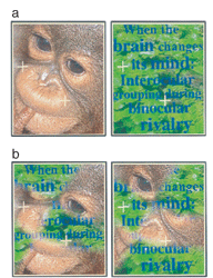
This animation simulates six, independent "zones" displaying portions of a monkey face or a jungle scene. The time-course of appearance within each zone was created using the procedure summarized below. Watching the animation, one sees occasional, striking periods of time during which the monkey face or the jungle scene is primarily dominant. Indeed, the animation does a remarkably good job of simulating rivalry observed with IOG display shown at the left, especially considering that the six dynamic image fragments are generated independently. Of course, the montage’s appearance will vary dependent on the size and distribution of the virtual zones, but the values selected are not unreasonable given our knowledge of the sizes of spatial zones of rivalry measured empirically (Blake et al, 1992). |
|
|
|
Dichoptic displays inducing binocular rivalry. (a) Conventional displays consisting of "whole" monocular images. (b) Displays consisting of complementary, patchy images. Complete dominance of the monkey or the jungle scene in the "patchy" display conclusively demonstrates interocular grouping. (Reproduced, with permission, from Kovacs et al, 1996)
|
|
|
 |
|
|
|
 |
|
|
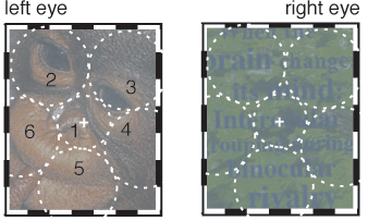
The display were segmented into six, circularly shaped virtual regions around the fixation cross. The radius was .67 deg for the region at the fixation (‘1’) and 1 deg for the other regions (‘2’~’6’).
|
|
|
|
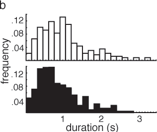
Histograms of dominance durations are shown for the monkey (top), jungle (bottom) percepts in local zone ‘2’
|
|
|
|
 |
|
|
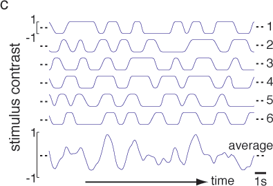
| Each of the six graphs to the left shows an example of fluctuations of image contrast over time for patches of rival images within each local region of the display in the hybrid animation. A value ‘1’ means that the contrast of a patch of monkey face is its original value while the contrast of a patch of jungle scene is zero, and vice versa for a value ‘–1’. The 'average' graph at the bottom shows fluctuations of the mean contrast averaged across the six local regions. |
|
|
|
|
|
|
|
|
|
|
|
|
|
|
|
|
|
|
|
|
