Tutorial on Spatial Frequency Analysis
(This material was excerpted, in part, from Chapter Five of Perception, 3rd Edition, by Robert Sekuler and Randolph Blake. References and additional information can be found in that chapter. As well, you are referred to a wonderful website called the Joy of Visual Perception, authored by Peter Kaiser at York University. That electronic "text" has lots of good material on spatial vision and other topics we'll cover.)

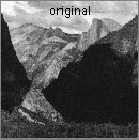
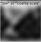
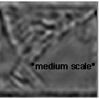
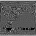
Shown below is a series of pictures of a natural scene. The one on the far left is the original, and the next three show this same scene at three different spatial scales: low, medium and high.

Regardless of the distance from which a scene is viewed, images of naturally occurring scenes or objects (trees, rocks, bushes, etc.) tend to contain information at many different spatial scales, from very fine to very coarse. the series of photographs shown above illustrate this point. The viewer's goals determine what component of this information is paramount. Because goals change, one scale may be more important than another now, but less important later. Sometimes it's important to see the forest; other times the trees, or the leaves, are essential. Ideally, then, your brain's neural representation of a scene would contain the information from all scales simultaneously. By having access to representations of scenes or objects at different spatial scales, the visual system can solve problems that would be intractable using a single representation. How does the visual system implement this multiple-scale representation?

The mammalian visual system is well suited to create neural representations of any visual scene simultaneously on several different scales. In principle, neurons with different sized receptive fields could capture the presence of borders or edges at different scales (recall that a neuron's receptive field is the region of the retina over which visual signals influence the activity of that neuron). Two British vision researchers, Fergus Campbell and John Robson, developed a theory of form perception in which the visual system would use neurons with different receptive field sizes to create a series of neural representations on different scales. Their theory, which has been subjected to numerous empirical tests, has been enormously influential.

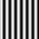
Campbell and Robson hypothesized that at different levels of the visual system, the responses of various neurons form a neural representation of the image falling on the retina. Because neurons' receptive fields vary in size, the responses of different subsets of neurons would constitute a neural representation at some particular scale. To test their hypothesis, Campbell and Robson needed stimuli whose orientation and size could be varied systematically. In addition, knowing that contrast is important in detection, they needed to specify and vary contrast as well. A stimulus such as the one shown below satisfies all these requirements. Such patterns, called gratings, can be generated on a television display. The one seen here is called a sinusoidal grating because the intensity of its light and dark bars changes gradually, in a sinusoidal fashion. At sufficiently low contrast, the television screen would appear uniform and unpatterned; at higher contrasts, the pattern would be visible. For various gratings, Campbell and Robson determined the minimum contrast necessary to see the grating, a value called the contrast threshold.

Using gratings they were able to prove that the visual system contains sets of neurons tuned to different bar widths. They called these sets of neurons channels, and because their theory relates form perception to activity within many such channels, it is known as the multichannel model. Let's consider grating patterns in greater detail.

GRATINGS AS TOOLS FOR
EXPLORING FORM PERCEPTION

What Exactly Are Gratings? Gratings have four properties -- spatial frequency, contrast, orientation, and spatial phase. These properties are independent of one another, in the sense that any one of them can be changed without affecting the others. Orientation is pretty easy to grasp - it simply refers to the tilt of the grating: vertical, horizontal, oblique. But we will have to consider the other three.

"Spatial frequency" refers to the number of pairs of bars imaged within a given distance on the retina. One-third of a millimeter is a convenient unit of retinal distance because an image this size is said to subtend one degree of visual angle on the retina. To give an example, your index fingernail casts an image of this size when that nail is viewed at arm's length; a typical human thumb, not just the nail, but the entire width, casts an image about twice as big, two degrees of visual angle. The size (or visual angle) of the retinal image cast by some object depends on the distance of that object from the eye; as the distance between the eye and an object decreases, the object's image subtends a greater visual angle. The unit employed to express spatial frequency is the number of cycles that fall within one degree of visual angle (each cycle is one dark and one light bar). A grating of high spatial frequency -- many cycles within each degree of visual angle -- contains narrow bars. A grating of low spatial frequency -- few cycles within each degree of visual angle -- contains wide bars. Because spatial frequency is defined in terms of visual angle, a grating's spatial frequency changes with viewing distance. As this distance decreases, each bar casts a larger image; as a result, the grating's spatial frequency decreases as the distance decreases.

"Contrast" is related to the intensity difference between the light and dark bars of the grating. If this difference is great, the grating's contrast is high; a small difference means the contrast is low. If the contrast is low enough, the bars of the grating may not even be visible. In this case, the grating contrast is said to be "below the threshold for visibility." Quantitatively, contrast runs from 0 percent (when there is no difference at all between the intensity of the light and dark bars) to 100 percent (when the difference between light and dark bars is maximum). The contrast of the print you are reading is about 70 percent; the contrast in the grating shown above is about 80 percent.

"Spatial phase" refers to a grating's position relative to some landmark (such as the edge of the television display). A convenient landmark is the left edge of the display. Looking at that edge, we can say that a grating "begins" with a dark bar, a light bar, or something in between.

Manipulating these four properties of a grating -- spatial frequency, contrast, orientation, and phase -- we can construct any visual pattern, even a human face. The visual image of a complex object or scene, in other words, is made up of a wide range of spatial frequencies and orientations. Normally we're not aware of those individual spatial frequency components, for our visual system blends them together into a single visual representation. But we can use computer-based "filtering" procedures to decompose a complex image into its constituent spatial frequencies. That's how the mountain scenes shown above were produced, and you'll be using filtering to produce this week's homework.

But before we advance to image filtering, you need to know how you can use gratings to measure the visual performance of your own visual system. To introduce this idea, consider first how you might measure the visual performance of a simpler optical device: a camera lens.

Using Gratings to Measure Performance Measuring a camera lens's performance requires two steps. First, we would use the lens to create an image of some target; then we would compare the image with the actual target. For example, using a lens, we would create an image of a grating of specified spatial frequency and contrast. We could then determine how good an image the lens had created. But "good" is an extremely vague term; how could we quantify it?

One approach is simply to judge the appearance of the image. But this subjective procedure can be misleading. A better, more objective way to assess the quality of images is by means of some physical instrument that measures light. The following example shows how this can be accomplished. Suppose we use an expensive, high-quality lens to cast, on a clean white paper, an image of a grating. We can use the light-measuring instrument to determine the contrast of the image produced by the lens. Let's repeat this for different spatial frequencies, always using gratings of the same contrast. We can graph the results in the following way. The horizontal axis of the graph will show spatial frequency; the vertical axis will show the image's contrast (as a percentage of the target's contrast). The resulting plot is often called a transfer function, because it specifies how contrast is transferred through the lens. Such a graph is shown below.

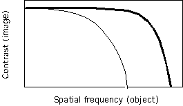
Look first at the heavy line in the graph. Note that up to a certain spatial frequency the contrast in the image is identical to that of the target. For these frequencies, the lens faithfully reproduces the target. However, for still higher spatial frequencies, the contrast in the image is reduced even though the contrast in the target is constant. For these spatial frequencies, the lens reproduces the target less faithfully. The frequency at which the image contrast falls to zero is called the cutoff frequency; once the frequency in an actual target exceeds this value, the image will no longer contain any contrast whatsoever -- the target itself might as well have zero contrast.

Notice the second curve in graph (the thin line). This curve connects the points we would observe if we repeated the experiment after having made one modification: smearing the lens by running a buttery finger over its surface. At very low spatial frequencies, the smear makes little difference in the performance of the lens. However, at intermediate spatial frequencies, the contrast in the image is degraded by the butter on the lens. This is shown by the difference between the curves for the lens in its buttered and unbuttered states. Note also that the cutoff frequency for the buttered lens is lower than that for the clean lens. This difference between the curves makes intuitive sense: a high-quality lens excels at imaging fine spatial detail and coarse spatial detail, while a low-quality lens images only the latter.

So, the transfer function of a lens summarizes its performance, although in a rather abstract way. In this respect, the transfer function serves the same purpose as the United States Environmental Protection Agency's (EPA) mileage ratings for various cars tested under standard conditions. While they are useful, the EPA ratings may not specify the performance of a car under particular driving conditions. By the same token, the curves in the graph do not indicate how any particular scene will appear on a photograph taken through that lens. They indicate only how the lens will handle one special set of "scenes" -- namely, gratings. But most people want to use their cameras to photograph things other than gratings. To see how transfer functions can be applied to photographing some scene, that scene must be related to gratings.

One method for doing exactly this comes from the work of Jean Baptiste Fourier, a nineteenth-century French mathematician. As part of a prestigious mathematics contest, Fourier was required to develop equations expressing how heat is transferred from one body to another. He recognized that extremely complex equations would be needed and that those equations would have to be general enough to apply to a wide variety of different bodies. To satisfy these requirements, Fourier developed a powerful simplification. He showed that if some quantity (such as heat) changed in a complex manner over time, that complex function of time could be approximated by a series of simple sinusoidal functions. This simplification was an enormous advantage because it allowed Fourier to break a mathematically difficult function down into simpler, mathematically more tractable components. From here the problem could be solved by working with the simple components (incidentally, he won the contest). In recognition of his accomplishment, we now refer to his technique as Fourier analysis. (For a brief, non-technical overview of Fourier analysis and gratings, see this website or this one; for more technical details on Fourier analysis, try this one.)

But how does Fourier's solution enable us to relate simple sinusoidal functions to a photograph of some scene taken through a lens? First, we can consider that scene as the sum of a series of simple sinusoidal components. Then, using the transfer function of the lens, we can evaluate how the lens would image each of those components. Consider the lens whose transfer function is given by the lighter line in the graph above (the lens smeared with butter). If we used that lens to photograph a scene containing many very fine details, the resulting image would be low in contrast and would appear very washed out. This is because "fine detail" is equivalent to "high spatial frequency." As the transfer function shows, the buttered lens does a poor job of transferring high spatial frequencies; it reduces the contrast of any high spatial frequencies contained in a scene. Though this lens could faithfully represent the general shape of a large target (such as a tree that is near the camera), it would not be adequate for fine details (such as the wrinkles in the tree's bark). This illustrates that sinusoidal targets can predict the quality of a photograph produced by a lens. To reiterate, several steps are involved. First, we determine the transfer function of the lens. Second, we analyze the visual scene into its spatial frequency components. With these pieces of information in hand, we determine which spatial frequency components will be preserved in the image of that scene and which will not. The second of these steps is mathematically complex, and we'll not worry with details. The first step, measuring the transfer function, is straightforward in the camera. But how easy is it to measure a transfer function for a visual system such as your own? If we did know your transfer function, we could better predict the visibility of scenes you might look at. Our next goal, then, is to derive a transfer function for human vision comparable to the one we derived for a lens.

THE CONTRAST SENSITIVITY FUNCTION
AS A WINDOW OF VISIBILITY

The Human Contrast Sensitivity Function There's one major stumbling block to measuring a transfer function for human vision: we cannot duplicate with humans the procedure employed with a lens. While we can produce sinusoidal gratings of known contrast, it's difficult to measure the image such gratings produce because that image is inside the eye. Anyway, measuring this image would give only part of the visual system's complete transfer function. While describing the eye's optical components, this transfer function would not reflect the neural components of the visual system. And since we are interested in visual perception, not just the image formed in the eye, we must be concerned with the perceptual transfer function, which depends both on the optical transfer function and on the neural transfer function.

How then can we measure the perceptual transfer function? If your visual system (both its optical and its neural components) did a good job of transferring some spatial frequency, it stands to reason that you'd need little contrast to see a grating of that frequency -- in other words, you'd be relatively sensitive to that frequency. However, if your visual system did a poor job of transferring that spatial frequency, you'd need more contrast to see it -- you'd be relatively insensitive to that frequency. In general, the sensitivity of the visual system determines the threshold contrast needed to detect a given spatial frequency. By measuring contrast thresholds for different spatial frequencies, we can derive a curve that describes the entire visual system's sensitivity to contrast. Let's call this curve the contrast sensitivity function (CSF), to distinguish it from the transfer function of a lens. The term "sensitivity" is a reminder that we are dealing with a property of the visual system, not just a property of the stimulus. As you'd expect from everyday usage of the term "sensitivity," someone is said to have high sensitivity if that person requires little contrast to see a pattern. By the same token, someone is said to have low sensitivity if that person requires considerable contrast to see a pattern. Defined in this way, sensitivity is inversely related to threshold contrast. By navigating to this webpage you can download an image for testing your own CSF:

http://totoro.berkeley.edu/izumi/CSF/A_JG_RobsonCSFchart.html

The CSF defines your window of visibility.

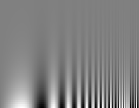
In the figure above, spatial frequency increases as you look from left to right (the bars become thinner and thinner) and contrast decreases as you look from bottom to top (bars become more difficult to see). From a fixed viewing distance, notice over the range of spatial frequencies the contrast values where the bars are just barely visible - imagine placing a curve along those points of threshold visibility. You'd trace out an inverted U-shaped curve. This is your contrast sensitivity function.

In the lab, here's how the CSF can be measured. A test grating is created electronically on a specially designed and calibrated television screen. The screen displayed a grating of fixed spatial frequency. Using a knob (like the contrast control on a television set), the contrast is adjusted until the grating is just visible. This threshold contrast is recorded by an experimenter. Typically, several estimates of the contrast threshold are measured for that spatial frequency and these estimates are averaged. This procedure is then repeated for other spatial frequencies, and the results are finally displayed as a curve that defines a window of visibility: the region below the curve represents combinations of contrast and spatial frequency that can be seen, while the region above the curve represents combinations that cannot be seen. To clarify this idea, pick any point on the CSF curve you traced out for yourself above. Because this point is the threshold contrast for seeing that pattern, decreasing the pattern's contrast (moving upward from the curve) renders the pattern invisible. Conversely, increasing the pattern's contrast (moving downward from the curve) makes the pattern more visible.

Note that in one respect the shape of the human CSF resembles the shape of the transfer function of a lens: each displays a high-frequency cutoff. However, in another respect the two are different. In particular, the CSF drops at low frequencies, whereas the lens's function does not. The visual system, in other words, is less sensitive to very low spatial frequencies than it is to intermediate ones. As a result, there is a range of spatial frequencies, toward the center of the horizontal axis, where humans are maximally sensitive. Gratings are less visible if they lie on either side of this optimum spatial frequency; a person requires higher contrast in order to see them. The same line of reasoning can be applied to a visual scene or photograph of that scene. If the objects in a scene have most of their spatial frequency information around the optimum point on the CSF, those objects will be clearly visible even when they are of low contrast. If those objects contain only very low spatial frequencies (very large objects) or only very high spatial frequencies (very small objects or fine details), they will be less visible and their contrast will have to be high in order for those objects to be seen.

You know from experience that you are able to see better under some conditions than others. If the CSF and your ability to see are importantly related, conditions that change one should also change the other. In fact, this is precisely what happens. Let's consider one such condition.

As we talked about when considering rods and cones, visual resolution is poor under dimlight conditions. That is why it's hard to read in dim light. Since resolution involves seeing fine detail, we'd expect decreased light to affect particularly that portion of the CSF corresponding to fine detail. Indeed this happens: As the level of light decreases from daylight to twilight, visual sensitivity drops primarily at high spatial frequencies; lower frequencies are little affected. But when the light falls to extremely low levels (nighttime), sensitivity decreases even at low frequencies. Think about what these curves imply for your vision under changing conditions of illumination. Driving at night, you may be unable to see the fine details (high frequencies) of the shrubs alongside the road. At the same time, you probably will be able to see larger objects (low frequencies), such as another car, just about as well as you do under daylight conditions. If you park your car in an unlit place and turn off your headlights, you will be operating under light conditions like those producing the scotopic curve. Under such conditions, even large objects will be difficult to see.

In summary, the CSF characterizes the ease with which people are able to detect objects of various sizes and perceive the structural detail, such as texture, of those objects. Conditions that alter the CSF, such as light level, change the visibility and appearance of objects. In a sense, these conditions thrust one into a different visual world. The article you read several weeks ago on cat vision illustrated how the CSF could be used to "guess" what the world might look like to another species. Let's apply the same reasoning to inquire about vision in the very young and the very old.

Age and the CSF How the world might appear to individuals at various points in their lifetimes? To begin, suppose while you are reading this book, someone puts a human infant on your lap. How does your visual world compare to that of the infant? This question, incidentially, has intrigued philosophers and parents for centuries.

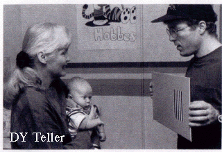
It is hard to know what very young, preverbal infants see. Obviously, you can't use the same methods to study infant vision that you use with cooperative, attentive adults. To get around this limitation, researchers have exploited a naturally occurring tendency exhibited by infants. It has been known for some time that an infant prefers to look at complex rather than dull scenes. Several research groups have exploited preferential looking to measure the infant's ability to see gratings. Shown below is a famous vision scientist - Davida Teller of Washington University - who has been instrumental in developing these baby testing procedures. The infant in her arms seems to be looking at the left-hand part of the test card, which is where a grating is located.

Confronted with a patch of grating and a patch of uniform brightness, an infant will prefer to look at the grating. If the infant shows no preference for the grating over the uniform field, it is inferred that the infant cannot see the grating. This could happen for one of two reasons: either the contrast of the grating is too low or the spatial frequency of the grating falls outside the range visible to the infant. The basic findings are summarized in the graph below, which shows CSFs for an infant somewhere between 3 to 6 months old and for a typical adult.

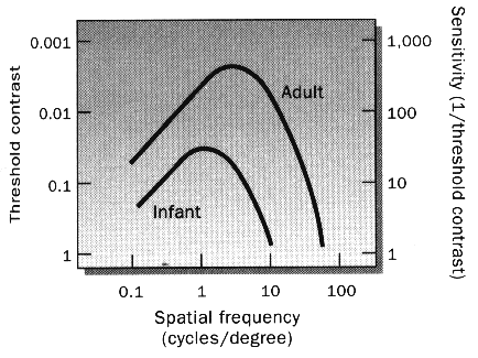
Note that the infant's window of visibility is very different from the adult's. An infant held on your lap will not be able to see fine spatial details visible to you. In this respect, the infant more closely resembles a cat. But unlike a cat, the infant does not have an advantage over you at low frequencies: you should be able to see everything that the infant can see. Also, even for spatial frequencies visible to both of you, the infant will require more contrast than you do. In a sense, these CSFs confirm what some parents have noticed: their very young infants seem oblivious to everything except very large, high-contrast objects. Incidentally, the lack of sensitivity to high frequencies does not stem from optical causes but from the fact that the infant's immature visual nervous system fails to encode high frequencies. In effect, infants are best suited for seeing objects located close to them (recall that spatial frequency is distance dependent), which makes sense from a behavioral standpoint.

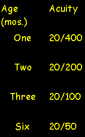
The infant's CSF improves gradually over the first year or so of its life - this means, among other things, that the infant/child's acuity gets better and better (see table below).

The improvement may be arrested, though, at an immature level if the infant does not receive normal visual experiences. There are several visual disorders that can alter the quality of visual experiences received by an infant and hence keep spatial vision from its normal course of development. First of all, any condition that chronically blurs the images reaching the infant's retina will limit the information available to the visual system. Optical blur of this sort can result from myopia or hyperopia and from congenital cataracts or corneal scars. Misalignment of an infant's two eyes can also retard the development of good spatial vision. When its eyes are not properly aligned, an infant must suppress or ignore visual input from one eye in order to avoid seeing double. For reasons unknown, continuous suppression of one eye can lead to a loss in spatial vision, a condition called amblyopia . Fortunately, infants afflicted with any of these disorders can recover normal spatial vision, providing that the disorder is corrected sometime during the first few years of life. But if correction is postponed until the child reaches school age, the prognosis for full recovery is much poorer. Apparently there is a critical period early in life when the visual nervous system requires normal input to mature properly. During this period, neural connections are still being formed. This critical period of neural development ends by the time a child reaches 3 or 4 years of age. If the visual nervous system arrives at this stage not completely developed because of inadequate visual experience, any neural abnormalities are irrevocably preserved throughout the remainder of life. In view of this critical role of early visual experience, you can appreciate the importance of detecting and correcting visual disorders in infants as early as possible. One important reason for studying infant vision is to develop and refine techniques allowing early diagnosis of such disorders.

So far our discussion has focused on spatial vision in infants and young children. Consider now what happens to the CSF during the remainder of the life span. The CSF remains more or less stable through young adulthood; but after age 30, systematic changes in the CSF begin reappearing.

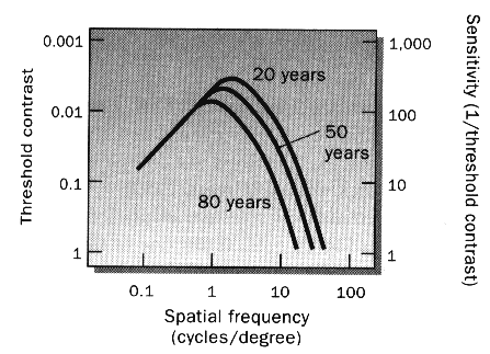
Specifically, there is a steady loss in high spatial frequency sensitivity, meaning that acuity is falling. Very likely much of the loss in sensitivity to high frequencies results from optical changes in elderly eyes. For example, as people grow older, their pupils become smaller, which means that their retinae receive considerably less light than yours. This reduced illumination of the retina mimics changes that would be seen in your CSF as you went from high to medium light levels. But whatever its origins, the variation in the CSF from birth to old age means that people experience very different visual worlds at different stages of their lives.

Some more notes on spatial vision can be found by navigating to this website.

Visual neurons have receptive fields (the region of the retina within which an image produces a change in the neuron's activity level). Different neurons have different sized receptive fields, ranging from very small to quite large. As you might expect, neurons registering visual information from the foveal area of the retina (where acuity is best) have small receptive fields - this allows them to register fine spatial detail. Receptive fields registering information in the periphery are larger, which explains in part why acuity is poorer in the periphery.

But at any given location of the visual field, we find a range of receptive field sizes. In other words, the image is being analyzed by neurons responsive to different spatial frequencies within that portion of the image falling on that part of the retina. To help you visualize what a receptive field does, think of a series of sieves with holes of different diameters, with one sieve stacked on top of the other. If you were to drop a bunch of marbles of different sizes into this series of sieves, the different sized holes would "filter" the balls according to size. In a sense, this is what visual neurons do at any given location of the retina: different sized receptive fields register image information at different spatial scales (where spatial scale refers to spatial frequency). The large holes correspond to low spatial frequencies, the small ones to high spatial frequencies.

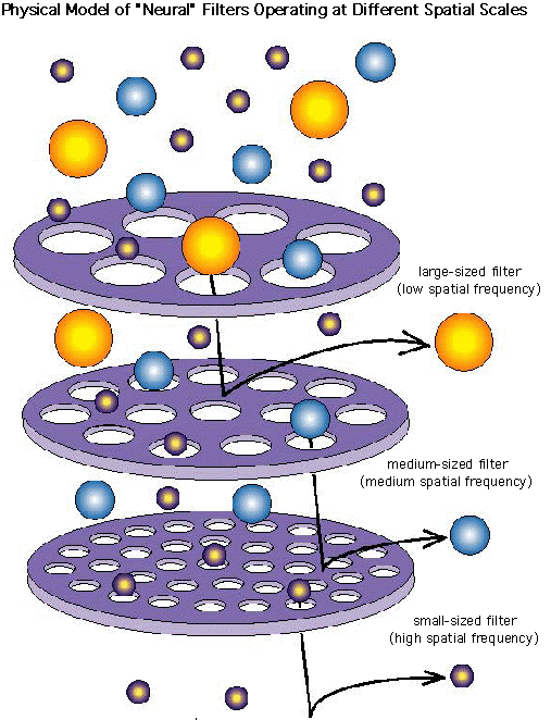
Looking back at the natural scene portrayed earlier, the "low" spatial frequencies would stimulate neurons with large receptive fields and the "high" spatial frequencies the neurons with small receptive fields.

Homework: this week in class you will use software to filter different spatial frequencies from natural images and from gratings.